이전에 만든 데이터세트를 가지고 모델을 만든다.
이전에 PyCaret을 통해 간단하게 모델들을 돌려봤는데, 가장 좋은 성능을 보여준 lightGBM, Gradient Boosting Classifier, Logisitic Regression을 중심으로 학습할 예정이다.
+ 임시로 돌려볼 모델들
# Pycaret으로 모델 돌려보기
# Pycaret 간단 정리
!pip install pycaret # model 비교 라이브러리 설치

from pycaret.classification import *

exp_clf = setup(data = train, target = 'y', session_id=123) # data setup 보기
models() # 사용되는 models 보기

best_model = compare_models() # 전체 모델 비교

lr = create_model('lr') # 특정 모델 비교
tuned_lr = tune_model(lr, n_iter=100, optimize='Accuracy') # 모델 튜닝
tuned_lr # 튜닝된 모델 파라미터 설정 보기
# XGBoost
dataset이 알맞게 전처리 됐는지 확인하기 위해 돌려본 모델!
앙상블모델이라 성능도 나쁘지 않을 것이고, 다른 팀원들과 겹치지 않게 선정했다.
# 데이터 나누기
X_features = train.iloc[:, :-1]
y_labels = train.iloc[:, -1]

y_labels = pd.Series(np.where(y_labels.values == 'yes', 1, 0), # label int형으로 변환(no->0, yes->1)
          y_labels.index)

from sklearn.model_selection import train_test_split

X_train, X_test, y_train, y_test = train_test_split(X_features, y_labels,
test_size=0.2, random_state=0)- 일단 모든 모델에서 해주어야 하는 것.
- 데이터를 feature와 label로 나눈다.
- 그리고 train_test_split() 함수를 이용해 데이터를 train/test로 나눈다.
from xgboost import XGBClassifier
from sklearn.metrics import f1_score, roc_auc_score, confusion_matrix, recall_score, precision_score, accuracy_score

# X_train, y_train을 다시 학습과 검증 데이터 세트로 분리. (조기중단)
X_tr, X_val, y_tr, y_val = train_test_split(X_train, y_train,
                                                    test_size=0.3, random_state=0)

# n_estimators는 500으로, learning_rate 0.05, random state는 예제 수행 시마다 동일 예측 결과를 위해 설정.
xgb_clf = XGBClassifier(n_estimators=500, learning_rate=0.05, random_state=156)

# 성능 평가 지표를 auc로, 조기 중단 파라미터는 100으로 설정하고 학습 수행.
xgb_clf.fit(X_tr, y_tr, early_stopping_rounds=100, eval_metric='auc', eval_set=[(X_tr, y_tr), (X_val, y_val)])- 조기 중단을 위해, train data를 다시 학습 데이터와 검증 데이터로 나눈다.
- XGBClassifier()로 학습 모델을 만든다.
- 모델 학습해주기. 평가 metrics는 auc로 했다. 왜인지는 모르겠는데 f1제공을 안해서...auc 아님 logloss로 한다고 함.
pred_probs = xgb_clf.predict(X_test) # 예측 확률값 반환
pred = [ 1 if x > 0.5 else 0 for x in pred_probs ] # 확률에 따라 label 변환

# f1-score는 확률 값으로 안됨.
xgb_roc_score = f1_score(y_test, pred, average= 'micro')
print('F1: {0:.4f}'.format(xgb_roc_score))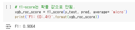
하이퍼 파라미터 튜닝을 따로 해주지 않았는데도 좋은 성능이 나왔다!
베이지안 최적화 기반으로 하이퍼 파라미터 튜닝을 해준다. GridSearch보다 빠름.
from hyperopt import hp # 하이퍼 파라미터 튜닝

# max_depth는 5에서 15까지 1간격으로, min_child_weight는 1에서 6까지 1간격으로
# colsample_bytree는 0.5에서 0.95사이, learning_rate는 0.01에서 0.2사이 정규 분포된 값으로 검색.

xgb_search_space = {'max_depth': hp.quniform('max_depth', 5, 15, 1),
                    'min_child_weight': hp.quniform('min_child_weight', 1, 6, 1),
                    'colsample_bytree': hp.uniform('colsample_bytree', 0.5, 0.95),
                    'learning_rate': hp.uniform('learning_rate', 0.01, 0.2)
}- 파라미터 범위 설정
from sklearn.model_selection import KFold
from sklearn.metrics import f1_score
from xgboost import XGBClassifier
import numpy as np

# 목적 함수 설정.
# 추후 fmin()에서 입력된 search_space값으로 XGBClassifier 교차 검증 학습 후 -1* f1_score 평균 값을 반환.
def objective_func(search_space):
    xgb_clf = XGBClassifier(n_estimators=100, max_depth=int(search_space['max_depth']),
                            min_child_weight=int(search_space['min_child_weight']),
                            colsample_bytree=search_space['colsample_bytree'],
                            learning_rate=search_space['learning_rate']
                           )
    # 3개 k-fold 방식으로 평가된 f1_score 지표를 담는 list
    f1_list = []

    # 3개 k-fold 방식 적용
    kf = KFold(n_splits=3)
    # X_train을 다시 학습과 검증용 데이터로 분리
    for tr_index, val_index in kf.split(X_train):
        # kf.split(X_train)으로 추출된 학습과 검증 index값으로 학습과 검증 데이터 세트 분리
        X_tr, y_tr = X_train.iloc[tr_index], y_train.iloc[tr_index]
        X_val, y_val = X_train.iloc[val_index], y_train.iloc[val_index]
        # early stopping은 30회로 설정하고 추출된 학습과 검증 데이터로 XGBClassifier 학습 수행.
        xgb_clf.fit(X_tr, y_tr, early_stopping_rounds=30, eval_metric='logloss',
                   eval_set=[(X_tr, y_tr), (X_val, y_val)])

        # 예측값 추출 후 f1_score 계산하고 평균 f1_score 계산을 위해 list에 결과값 담음.
        y_pred = xgb_clf.predict(X_val)
        score = f1_score(y_val, y_pred)
        f1_list.append(score)

    # 3개 k-fold로 계산된 f1_score값의 평균값을 반환하되,
    # HyperOpt는 목적함수의 최소값을 위한 입력값을 찾으므로 -1을 곱한 뒤 반환.
return -1 * np.mean(f1_list)- 목적 함수 설정
from hyperopt import fmin, tpe, Trials

trials = Trials()

# fmin()함수를 호출. max_evals지정된 횟수만큼 반복 후 목적함수의 최소값을 가지는 최적 입력값 추출.
best = fmin(fn=objective_func,
            space=xgb_search_space,
            algo=tpe.suggest,
            max_evals=50, # 최대 반복 횟수를 지정합니다.
            trials=trials, rstate=np.random.default_rng(seed=30))

print('best:', best)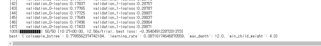
- 위 목적 함수와 범위 설정을 바탕으로 튜닝을 실행한다.
- 튜닝 결과는 best에 저장
# n_estimators를 500증가 후 최적으로 찾은 하이퍼 파라미터를 기반으로 학습과 예측 수행.
xgb_clf = XGBClassifier(n_estimators=500, learning_rate=round(best['learning_rate'], 5),
                        max_depth=int(best['max_depth']), min_child_weight=int(best['min_child_weight']),
                        colsample_bytree=round(best['colsample_bytree'], 5)
                       )

# evaluation metric을 auc로, early stopping은 100 으로 설정하고 학습 수행.
xgb_clf.fit(X_tr, y_tr, early_stopping_rounds=100,
            eval_metric="logloss",eval_set=[(X_tr, y_tr), (X_val, y_val)]) # logloss : 0.9008, auc : 0.9021

pred_probs = xgb_clf.predict(X_test) # 예측 확률값 반환
pred = [ 1 if x > 0.5 else 0 for x in pred_probs ] # 확률에 따라 label 변환

# f1-score는 확률 값으로 안됨.
xgb_roc_score = f1_score(y_test, pred, average= 'micro')
print('F1: {0:.4f}'.format(xgb_roc_score))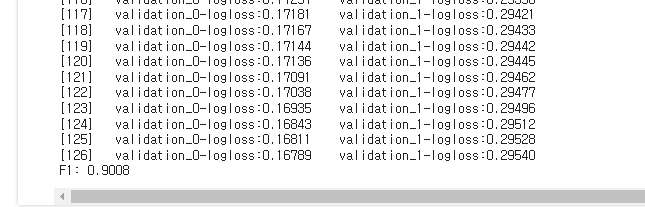
- 성적이 더 떨어졌...learning rate를 0.05에서 0.2로 늘린게 큰 듯. 시간이 좀 더 오래 걸리더라도 값을 작게 해보자.
- 또 eval_metric을 logloss가 아닌 auc로 할 때 더 성능이 잘 나오는 것 같기도 하다. 왜지?
# LightGBM
lgbm_search_space = {'num_leaves': hp.quniform('num_leaves', 32, 64, 1),
                     'max_depth': hp.quniform('max_depth', 100, 160, 1),
                     'min_child_samples': hp.quniform('min_child_samples', 60, 100, 1),
                     'subsample': hp.uniform('subsample', 0.7, 1), # 추가
                     'learning_rate': hp.uniform('learning_rate', 0.01, 0.2)
}- search_spave에 subsample을 추가했다.
# !pip install lightgbm==3.3.2
import re
train = train.rename(columns = lambda x:re.sub('[^A-Za-z0-9_]+', '', x))# lightgbm이 특수문자를 인식 못함..;;- LGBMClassifier.fit() got an unexpected keyword argument 'early_stopping_rounds' 오류 발생
- lgbm이 4.x로 업그레이드 되면서 파라미터가 좀 수정된 듯. 3.3.2로 낮추었다.
- Do not support special JSON characters in feature name. 오류 발생
- lightgbm은 특수문자 처리를 못해서;;; 위와 같이 feature name을 수정했다.
from sklearn.model_selection import KFold
from sklearn.metrics import roc_auc_score
from lightgbm import LGBMClassifier

def objective_func(search_space):
    lgbm_clf =  LGBMClassifier(n_estimators=100, num_leaves=int(search_space['num_leaves']),
                               max_depth=int(search_space['max_depth']),
                               min_child_samples=int(search_space['min_child_samples']),
                               subsample=search_space['subsample'],
                               learning_rate=search_space['learning_rate'])
    # 3개 k-fold 방식으로 평가된 roc_auc 지표를 담는 list
    roc_auc_list = []

    # 3개 k-fold방식 적용
    kf = KFold(n_splits=3)
    # X_train을 다시 학습과 검증용 데이터로 분리
    for tr_index, val_index in kf.split(X_train):
        # kf.split(X_train)으로 추출된 학습과 검증 index값으로 학습과 검증 데이터 세트 분리
        X_tr, y_tr = X_train.iloc[tr_index], y_train.iloc[tr_index]
        X_val, y_val = X_train.iloc[val_index], y_train.iloc[val_index]

        # early stopping은 30회로 설정하고 추출된 학습과 검증 데이터로 XGBClassifier 학습 수행.
        lgbm_clf.fit(X_tr, y_tr, early_stopping_rounds=30, eval_metric="auc",
           eval_set=[(X_tr, y_tr), (X_val, y_val)])

        # 1로 예측한 확률값 추출후 roc auc 계산하고 평균 roc auc 계산을 위해 list에 결과값 담음.
        score = roc_auc_score(y_val, lgbm_clf.predict_proba(X_val)[:, 1])
        roc_auc_list.append(score)

    # 3개 k-fold로 계산된 roc_auc값의 평균값을 반환하되,
    # HyperOpt는 목적함수의 최소값을 위한 입력값을 찾으므로 -1을 곱한 뒤 반환.
return -1*np.mean(roc_auc_list)- 목적 함수 lgbm으로 수정
from hyperopt import fmin, tpe, Trials

trials = Trials()

# fmin()함수를 호출. max_evals지정된 횟수만큼 반복 후 목적함수의 최소값을 가지는 최적 입력값 추출.
best = fmin(fn=objective_func, space=lgbm_search_space, algo=tpe.suggest,
            max_evals=50, # 최대 반복 횟수를 지정합니다.
            trials=trials, rstate=np.random.default_rng(seed=30))

print('best:', best)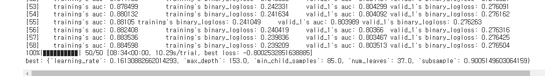
- 호출!
from lightgbm import LGBMClassifier

lgbm_clf =  LGBMClassifier(n_estimators=500,
                           max_depth=int(best['max_depth']),
                           min_child_samples=int(best['min_child_samples']),
                           subsample=round(best['subsample'], 5),
                           learning_rate=round(best['learning_rate'], 5),
                           num_leaves=int(best['num_leaves'])
                          )

# evaluation metric을 auc로, early stopping은 100 으로 설정하고 학습 수행.
lgbm_clf.fit(X_tr, y_tr, early_stopping_rounds=100,
            eval_metric="auc",eval_set=[(X_tr, y_tr), (X_val, y_val)])

# roc-auc
lgbm_roc_score = roc_auc_score(y_test, lgbm_clf.predict_proba(X_test)[:,1])
print('ROC AUC: {0:.4f}'.format(lgbm_roc_score))

# f1score
pred_probs = lgbm_clf.predict(X_test) # 예측 확률값 반환
pred = [ 1 if x > 0.5 else 0 for x in pred_probs ] # 확률에 따라 label 변환

# f1-score는 확률 값으로 안됨.
lgbm_f1_score = f1_score(y_test, pred, average= 'micro')
print('F1: {0:.4f}'.format(lgbm_f1_score))
# Random Forest
from hyperopt import hp

rfc_search_space = {
    'n_estimators': hp.quniform('n_estimators', 100, 1000, 100),
    'max_depth': hp.quniform('max_depth', 3, 20, 1),
    'min_samples_split': hp.quniform('min_samples_split', 2, 20, 1),
    'min_samples_leaf': hp.quniform('min_samples_leaf', 1, 20, 1),
    'max_features': hp.choice('max_features', ['auto', 'sqrt', 'log2', None]),
    'bootstrap': hp.choice('bootstrap', [True, False])
}
from imblearn.ensemble import BalancedBaggingClassifier
from sklearn.ensemble import RandomForestClassifier
from sklearn.metrics import f1_score
from sklearn.model_selection import KFold
import numpy as np
def objective_func(search_space):
base_clf = RandomForestClassifier(
n_estimators=100,
max_depth=int(search_space['max_depth']),
min_samples_split=int(search_space['min_samples_split']),
min_samples_leaf=int(search_space['min_samples_leaf']),
max_features=search_space['max_features'],
bootstrap=search_space['bootstrap'],
random_state=42
)
bagging_clf = BalancedBaggingClassifier(base_estimator=base_clf, n_estimators=10, random_state=42)
kf = KFold(n_splits=3)
f1_scores = []
for train_index, val_index in kf.split(X_train):
X_tr, X_val = X_train.iloc[train_index], X_train.iloc[val_index]
y_tr, y_val = y_train.iloc[train_index], y_train.iloc[val_index]
bagging_clf.fit(X_tr, y_tr)
preds = bagging_clf.predict(X_val)
f1 = f1_score(y_val, preds, average='micro')
f1_scores.append(f1)
return -np.mean(f1_scores)from hyperopt import fmin, tpe, Trials
trials = Trials()
best = fmin(fn=objective_func, space=rfc_search_space, algo=tpe.suggest, max_evals=100, trials=trials)
print("Best hyperparameters:", best)import numpy as np
from sklearn.ensemble import RandomForestClassifier
from sklearn.metrics import roc_auc_score, f1_score
from sklearn.model_selection import train_test_split
from imblearn.ensemble import BalancedBaggingClassifier
# 설정된 최적의 하이퍼파라미터
best_params = {
'n_estimators': 500,
'max_depth': int(best['max_depth']),
'min_samples_split': int(best['min_samples_split']),
'min_samples_leaf': int(best['min_samples_leaf']),
'max_features': best['max_features'],
'bootstrap': best['bootstrap']
}
# Random Forest Classifier 모델 초기화
rf_clf = RandomForestClassifier(
n_estimators=best_params['n_estimators'],
max_depth=best_params['max_depth'],
min_samples_split=best_params['min_samples_split'],
min_samples_leaf=best_params['min_samples_leaf'],
max_features=best_params['max_features'],
bootstrap=best_params['bootstrap'],
random_state=42
)
# BalancedBaggingClassifier 사용하여 클래스 불균형 해결
bagging_clf = BalancedBaggingClassifier(base_estimator=rf_clf, n_estimators=10, random_state=42)
# 학습 수행
bagging_clf.fit(X_train, y_train)
# roc-auc 점수 계산
rf_roc_score = roc_auc_score(y_test, bagging_clf.predict_proba(X_test)[:, 1])
print('ROC AUC: {0:.4f}'.format(rf_roc_score))
# f1-score 계산
pred = bagging_clf.predict(X_test)
rf_f1_score = f1_score(y_test, pred, average='micro')
print('F1: {0:.4f}'.format(rf_f1_score))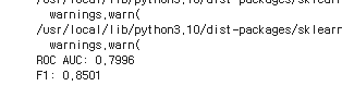
# GBC & Logistic Regression
이 두개를 왜 묶어 놨나면...둘다 간단하게 돌렸는데 f1 score가 0이 나왔다....
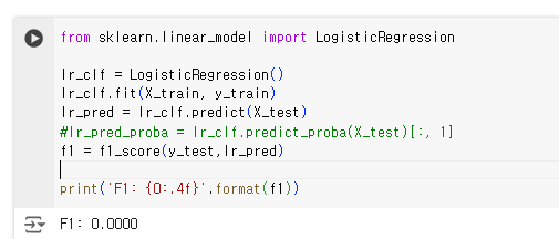
헉..다른 평가 방법으로도 돌려봤다.
from sklearn.metrics import confusion_matrix, accuracy_score, precision_score, recall_score, f1_score
from sklearn.metrics import roc_auc_score

# 평가 한번에 하는 함수^^7
def get_clf_eval(y_test, pred=None, pred_proba=None):
    confusion = confusion_matrix( y_test, pred)
    accuracy = accuracy_score(y_test , pred)
    precision = precision_score(y_test , pred)
    recall = recall_score(y_test , pred)
    f1 = f1_score(y_test,pred)
    # ROC-AUC 추가
    roc_auc = roc_auc_score(y_test, pred_proba)
    print('오차 행렬')
    print(confusion)
    # ROC-AUC print 추가
    print('정확도: {0:.4f}, 정밀도: {1:.4f}, 재현율: {2:.4f},\
    F1: {3:.4f}, AUC:{4:.4f}'.format(accuracy, precision, recall, f1, roc_auc))
from sklearn.linear_model import LogisticRegression
lr_clf = LogisticRegression()
lr_clf.fit(X_train, y_train)
lr_pred = lr_clf.predict(X_test)
lr_pred_proba = lr_clf.predict_proba(X_test)[:, 1]
get_clf_eval(y_test, lr_pred, lr_pred_proba)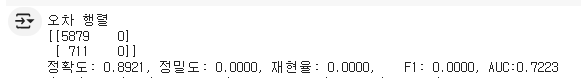
음...이렇게 나오는건 데이터셋이 불균형해서라고 생각함.
실제로 target값의 비율을 보니 불균형하긴 했다..!
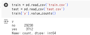
이런 경우 임계값을 조정하거나(default는 0.5로 알고 있음) unbalanced할 때 사용하는 파라미터를 이용하거나...할 수 있다.
그것까지 포함하여 튜닝을 진행한다.
# logistic regression
from hyperopt import hp

logreg_search_space = {
    'C': hp.loguniform('C', -4.0, 4.0),  # C 값은 0.018에서 약 54.6 사이의 값을 가질 수 있음
    'penalty': hp.choice('penalty', ['l1', 'l2']),
    'solver': hp.choice('solver', ['liblinear', 'saga'])  # l1 penalty를 위해 필요한 solver
}

# Example of how to use this search space with Logistic Regression
from hyperopt import fmin, tpe, Trials
from sklearn.linear_model import LogisticRegression
from sklearn.model_selection import cross_val_score
import numpy as np

def objective_func(search_space):
    logreg_clf = LogisticRegression(
        C=search_space['C'],
        penalty=search_space['penalty'],
        solver=search_space['solver'],
        max_iter=1000
    )

    # Using cross-validation to evaluate the model
    scores = cross_val_score(logreg_clf, X_train, y_train, cv=3, scoring='f1')
    return -np.mean(scores)  # Hyperopt minimizes the objective function

trials = Trials()
best = fmin(fn=objective_func, space=logreg_search_space, algo=tpe.suggest, max_evals=100, trials=trials)

print("Best hyperparameters:", best)- 반복 작업...search space와 objective func만 고쳐주기.

from sklearn.linear_model import LogisticRegression
from sklearn.metrics import roc_auc_score, f1_score
from sklearn.model_selection import train_test_split
from sklearn.utils.class_weight import compute_class_weight
# 설정된 최적의 하이퍼파라미터
best_params = {
'C': best['C'],
'penalty': ['l1', 'l2'][best['penalty']],
'solver': ['liblinear', 'saga'][best['solver']]
}
# 클래스 가중치 계산 -> 데이터세트 불균형 해소..
class_weights = compute_class_weight(class_weight='balanced', classes=np.unique(y_train), y=y_train)
class_weight_dict = dict(zip(np.unique(y_train), class_weights))
# Logistic Regression 모델 초기화 및 학습
logreg_clf = LogisticRegression(
C=best_params['C'],
penalty=best_params['penalty'],
solver=best_params['solver'],
max_iter=1000,
class_weight=class_weight_dict, # 클래스 가중치 적용
)
# 학습 수행
logreg_clf.fit(X_tr, y_tr)
# roc-auc 점수 계산
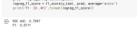
logreg_roc_score = roc_auc_score(y_test, logreg_clf.predict_proba(X_test)[:, 1])
print('ROC AUC: {0:.4f}'.format(logreg_roc_score))
# f1-score 계산
pred = logreg_clf.predict(X_test)
logreg_f1_score = f1_score(y_test, pred, average='micro')
print('F1: {0:.4f}'.format(logreg_f1_score))- Logistic Regression에서는 클래스 가중치를 계산 후 추가하는 방식으로 데이터 세트의 불균형을 해소한다.
# Gradient Boosting Classifier
from hyperopt import hp

gbc_search_space = {
    'learning_rate': hp.uniform('learning_rate', 0.01, 0.2),
    'max_depth': hp.quniform('max_depth', 3, 10, 1),
    'min_samples_split': hp.quniform('min_samples_split', 2, 20, 1),
    'min_samples_leaf': hp.quniform('min_samples_leaf', 1, 20, 1),
    'subsample': hp.uniform('subsample', 0.7, 1.0)
}
from imblearn.ensemble import BalancedBaggingClassifier
from sklearn.ensemble import GradientBoostingClassifier
from sklearn.metrics import f1_score
from sklearn.model_selection import KFold
import numpy as np

def objective_func(search_space):
    base_clf = GradientBoostingClassifier(
        n_estimators=100,
        learning_rate=search_space['learning_rate'],
        max_depth=int(search_space['max_depth']),
        min_samples_split=int(search_space['min_samples_split']),
        min_samples_leaf=int(search_space['min_samples_leaf']),
        subsample=search_space['subsample']
    )

    bagging_clf = BalancedBaggingClassifier(base_estimator=base_clf, n_estimators=10, random_state=42)

    kf = KFold(n_splits=3)
    f1_scores = []

    for train_index, val_index in kf.split(X_train):
        X_tr, X_val = X_train.iloc[train_index], X_train.iloc[val_index]
        y_tr, y_val = y_train.iloc[train_index], y_train.iloc[val_index]

        bagging_clf.fit(X_tr, y_tr)
        preds = bagging_clf.predict(X_val)
        f1 = f1_score(y_val, preds, average='micro')
        f1_scores.append(f1)

    return -np.mean(f1_scores)
from hyperopt import fmin, tpe, Trials
trials = Trials()
best = fmin(fn=objective_func, space=gbc_search_space, algo=tpe.suggest, max_evals=100, trials=trials)
print("Best hyperparameters:", best)
- GBC는 클래스 가중치 조절 파라미터가 따로 없어 BalancedBaggingClassifier라는 클래스 가중치를 조절하는 모델에 래핑하는 방식으로 조절한다.
from sklearn.ensemble import GradientBoostingClassifier
from sklearn.metrics import roc_auc_score, f1_score
from sklearn.model_selection import train_test_split

# 설정된 최적의 하이퍼파라미터
best_params = {
    'n_estimators': 500,
    'max_depth': int(best['max_depth']),
    'min_samples_split': int(best['min_samples_split']),
    'min_samples_leaf': int(best['min_samples_leaf']),
    'subsample': round(best['subsample'], 5),
    'learning_rate': round(best['learning_rate'], 5)
}

# Gradient Boosting Classifier 모델 초기화 및 학습
gb_clf = GradientBoostingClassifier(
    n_estimators=best_params['n_estimators'],
    max_depth=best_params['max_depth'],
    min_samples_split=best_params['min_samples_split'],
    min_samples_leaf=best_params['min_samples_leaf'],
    subsample=best_params['subsample'],
    learning_rate=best_params['learning_rate']
)

# 학습 수행
gb_clf.fit(X_tr, y_tr)

# roc-auc 점수 계산
gb_roc_score = roc_auc_score(y_test, gb_clf.predict_proba(X_test)[:, 1])
print('ROC AUC: {0:.4f}'.format(gb_roc_score))

# f1-score 계산
pred = gb_clf.predict(X_test)
gb_f1_score = f1_score(y_test, pred, average='micro')
print('F1: {0:.4f}'.format(gb_f1_score))
어쨌든 좋은 성능을 보여주지는 못함.
# 최종
가장 좋은 성능이 나온 모델을 선정하였다.
마지막까지 돌려본 모델은 모두 앙상블 기법 기반의 Random Forest, LightGBM, XGBoost였다.
이 3개의 모델들이 불균형한 데이터 세트에 좋다고 함.
결과는... XGBoost 선정! F1 score 0.9057로 가장 좋은 성능을 보여주었다.
이제 이 모델 학습 후 test 데이터를 예측할 것이다.
test데이터도 train 데이터와 마찬가지로 데이터 전처리를 해주어야 한다. feature가 똑같아야 함!
# test 데이터도 train처럼 변환
test = pd.read_csv('test.csv')
# 1. 데이터 drop
test.drop(['id','euribor3m', 'emp.var.rate'], axis=1 , inplace=True)
from sklearn.preprocessing import MinMaxScaler, StandardScaler, RobustScaler

# 2. 수치형 데이터 정규화
scaler = MinMaxScaler()
test[test.select_dtypes(include=np.number).columns.tolist()]=scaler.fit_transform(test[test.select_dtypes(include=np.number).columns.tolist()])

# 3. 카테고리형 데이터 결측치 최빈값으로 대체
test = test.replace('unknown', test.mode().iloc[0])

# 4. 카테고리형 데이터 원-핫 인코딩
test = pd.get_dummies(test, dtype=int)

# 데이터 rename
import re
test = test.rename(columns = lambda x:re.sub('[^A-Za-z0-9_]+', '', x))

# test data에는 default feature에 yes가 없으므로 인코딩이 안됨. 넣어주기
test['default_yes'] = 0
# 열 순서 재조정: 원래 열 순서에 'default_yes'를 특정 위치에 삽입 -> default_no 뒤에 넣어주기
columns = list(test.columns)
default_no_index = columns.index('default_no')  # 'default_no' 열의 인덱스를 찾음
columns.insert(default_no_index + 1, columns.pop(columns.index('default_yes')))  # 'default_yes' 열을 'default_no' 바로 뒤로 이동

# 재정렬된 열 순서를 사용하여 데이터프레임 재구성
test = test[columns]- 이때 test데이터의 defaute feature에는 no만 있어서, 원-핫 인코딩을 적용할 때 default_yes가 만들어지지 않았다.
- 데이터 추가하고 순서도 train이랑 똑같이 맞춰줌...ㅎㅎ
pred_probs = xgb_clf.predict_proba(test)[:, 1]  # 예측 확률값 반환
pred = [1 if x > 0.5 else 0 for x in pred_probs]  # 확률에 따라 label 변환

# 다시 test 데이터를 불러오고(drop 및 변환한 데이터 가져오기) y_predict 추가
# 예측 결과를 test 데이터프레임에 새로운 열로 추가
test = pd.read_csv('test.csv')
test['y_predict'] = pred

# 결과를 CSV 파일로 저장
test.to_csv('prediction.csv', index=False)- 분류한 값을 원본 데이터에 붙여서 결과 csv 파일을 만들어준다.
print(test.value_counts('y_predict'))
test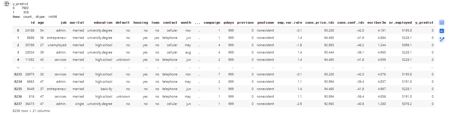
# 회고
이번 기회로 특히 하이퍼 파라미터 튜닝방식에 대해 많이 배웠다.
그동안 줄여서 파라미터라고 말했는데 따지면 그렇게 말하면 안되고...
GridSearchCV vs HyperOPT vs optuna 이 3개가 가장 많이 쓰이는 것 같다.
GridSearch는 당연하지만 성능이 가장 안좋음. 내가 설정한 파라미터 내에서만 하기 때문!
HyperOpt는 범위 내, 예를 들어 3, 10, 0.2로 설정하면 0.2 단위로 올려가며 최적 하이퍼 파라미터를 찾아가기 때문에 훨씬 정확하다.
optuna도 튜닝 자체는 비슷하지만, 다양한 모델에 적용 가능하며 여러 메소드를 지원해 편리하다.
optuna..이거 쓸 걸...까먹고 있다가 마지막에 생각났다ㅜ 다음에는 이걸로 도전!
힘들었다...! 진짜 여러 모델을 돌리니까 어렵다. 그나마 학습 과정을 통일해서 괜찮았던 것 같다.
'기타' 카테고리의 다른 글
| 정기 예금 가입 여부 예측 데이터 다루기 (0) | 2024.05.22 |
|---|---|
| Git 관리하자 (0) | 2024.04.12 |
| [AWS] AWS Public IPv4 주소 요금 변경2 + Q&A (0) | 2024.03.14 |
| [AWS] AWS Public IPv4 주소 요금 변경 + 문의 (0) | 2024.03.07 |
| 인류문명과환경공학 정리 (0) | 2024.01.09 |


